Upstream Oil and Gas Losses

In this briefing, we discuss various considerations in upstream oil and gas production losses, and in particular how rates of production depend on the type of well.  We also discuss what the shift to horizontal drilling and hydraulic fracturing means for calculating losses in the future and its other implications.

Measuring Lost Production

Calculating an upstream oil and gas loss starts with determining the loss of production.  Lost production is the difference between the production but for the loss incident (projected production) and actual production.

Projected production needs to be first determined for the well(s) in question by determining the production rate (i.e. the volume of oil or natural gas that is extracted per day) but for the loss.

Oil or gas wells are finite-life assets; as hydrocarbons are extracted and the formation is depleted, the production rate declines.  Therefore, unless the outage in question extends for a short period of time, a well’s declining production rate curve should be considered in projecting production but for the loss incident (“decline curve”).

Decline Curves

After the initial build-up in production rates and the plateau period that follows, the production rate of a well starts to decrease.  The rate of decline over time varies depending on many factors, the most significant of which is the type of well.

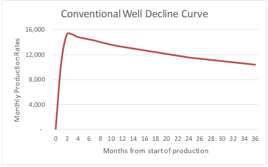
Historically, most wells were conventionally drilled vertical wells.  The decline curves on such wells were described to have an “exponential decline” which is generally a smooth curve over time, as shown in the graph below.  This is largely due to the permeable nature of the formation and the method of drilling.  Today, the Permian Basin is the play [1] with some significant legacy vertical production in the US.

The graph above mimics what a typical decline curve for a vertical Permian Basin well would look like, assuming a well would peak at 500 BBL per day [2]. In this example, the first year’s decline was 13% [3].

In contrast to conventional wells, drilling of unconventional wells typically combines horizontal drilling and hydraulic fracturing (“fracking”), and is aimed at low permeability formations that were previously inaccessible and uneconomic.  For oil reservoirs, these formations are known as “shale oil” and/or “tight oil”.  When such a formation is fracked, the initial production rate is high but prone to a steep decline.  This decline curve is characterized as a “hyperbolic decline”, as shown in the graph below.

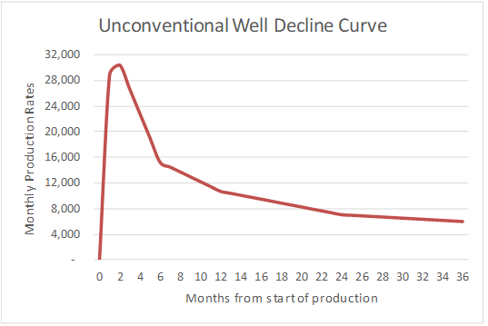
Most of the wells drilled in the US in the last 10 years are unconventional wells. The well above shows a typical production rate curve over the first 3 years of an unconventional well in the Bakken formation (based on a 2015 review published on Reuters [4]). By the end of the first year, production rates can be down 65% or more, and after three years, an average well will have already produced half of its lifetime production.  Although subsequent fracks can reinvigorate the production rate of an unconventional well for a time, the same dwindling production rate trend will repeat itself going forward.

What does the shift to horizontal drilling and hydraulic fracturing mean going forward? Average decline curves will continue to become steeper.  If the US intends to maintain domestic production and be self-sufficient in satisfying oil demand at home, US producers will have to keep drilling.

Offsetting the trend in steepening decline curves is the growing productivity of horizontal wells, achieved with technological advances allowing to drill further out horizontally, frack multiple sections, all resulting in a greater yield per well than previously possible.

Based on the above combination of factors influencing rates of production, a real-life well’s decline curve is sometimes an amalgam of the exponential and hyperbolic decline curves, depending on the well’s life stage, type of formation and type of well. It is modelled using complex engineering software. Often, a discussion with a petroleum engineer of the company that experienced an outage will help understand the well(s) in question and the production trends in relation to the entire field.

In summary, when quantifying an upstream loss, knowing the type of each well in question and where it is in its life cycle is key to projecting production.

There are, however, other significant factors to consider. Some of these factors are briefly outlined below.

Other Considerations in Projecting Production

Well / field pressure

Depending on the age of the field, the number of wells and the average wellhead pressure, the impact of an outage will be different.  Older fields extracting resources from an aged formation will have lower pressure and lower overall production.  A change in pressure due to a multiple-well outage may cause a substantially different impact than a change in pressure due to a single-well outage.

In addition, the degree of interrelationship between wells, i.e. how close they are located to each other, may determine how prone other wells’ production will be to change when certain wells are shut in (i.e., closed off and not producing).

Flush production

A common term that is used in discussing oil and gas production losses is “flush production”. Setting aside the differences in considering how the post-loss period of operations should be considered in a loss calculation, flush production occurs as a result of pressure buildup during the period the impacted well is shut in.  Largely depending on the length of the shut in, how many other wells were shut in, and the interrelationship between these wells, other wells may also experience some impact of flush production. It is important to consider whether this increase is a form of mitigation upon resumption of production following the loss incident.

Well reactivation and improvement

With the rise of unconventional drilling, more old wells are being reactivated and improved using more modern equipment.  For gas wells, this may involve installation of additional separation and field compression equipment, which helps improve production rates temporarily.

Well curtailment due to maintenance or overhaul

Any planned maintenance or overhaul needs to be considered. This has to be considered for the entire field, as often overhauling wells or even reactivating older wells requires a pipeline blow down to be completed, which may cause short-term shut ins of other wells.

Choked wells

Sometimes wells are not producing at capacity and are “choked”.  Choking a well means cutting back production by closing a choke which is a type of valve.  This may happen for various reasons; most commonly this occurs with new wells or if the capacity of the downstream facility is at maximum and cannot accept any more raw production.  In a loss calculation scenario considering new wells, a potential of them being choked sometimes needs to be factored in.

Technology advances

Decline curves are a snapshot at a point of time.  They often do not take into account labour, equipment, and other technology advances, which can extend the plateau stage of production or make the decline curve slope more gradual.

In summary, a proper approach to prepare a projection for well production in an upstream loss begins with the consideration of the well’s decline curve and includes a whole variety of quantitative and qualitative considerations.

Projecting Production for New Wells

Projecting production for a new well that was shut in as a result of an incident can be challenging.  Production engineers can use decline curves from an offset well to project production of a new well before it is completed or even drilled.  An offset well is a wellbore close to a proposed new well, which provides information for planning the proposed well.  Data that is obtained from an offset well can be often helpful in determining the necessary approach to drilling or treating the proposed new well, and to provide an indication of the decline curve of a new well.

Converting Lost Production to Lost Profit

After the production is projected, and actual production, if any, is considered, a shortfall in production is determined. It then needs to be priced (another commonly referred term is “monetized”) and reduced for the saved costs associated with the lost production, to arrive at the value of a net upstream loss.  Below are several common considerations.

Pricing

For simplicity, often some sort of actual average or historical average pricing is used to monetize the production loss.

The issue with this approach is that it often ignores price fluctuations which may change drastically day to day, depending on multiple factors including supply and demand, transportation capacity availability, political environment etc.  Actual pricing with the same level of granularity as the production loss calculation (e.g. daily pricing) will often present a truer value of monetized production loss.

Saved Costs Considerations

Average Costing

Echoing the issue of using averages above, saved costs are often calculated as the average of historical costs per unit of production.  The issue with averaging, in this case, is that the saved cost per unit of lost production may not be the average cost, but a marginal cost that would be incurred on marginal lost production.  Therefore, the saved costs associated with lost production may be materially different from the average cost, as discussed below.

Royalties

Royalties regimes will vary by jurisdiction. Royalty rates may also vary depending on levels of prices, cumulative well production to date, the time of drilling a well, the type of extracted hydrocarbon, and various well properties.  Using royalty rates from other wells or prior years as a benchmark may not be appropriate.

Transportation Costs

Transportation can occur by several modes under completely different cost ranges – from pipeline transportation to rail and truck. It is crucial to understand how the production that was lost would have been transported; this can often be done by determining how transportation of actual production changed following the incident causing the production loss.

If the business is able to optimize its costs, often the highest level of transportation cost is avoided as a result of a loss; therefore, using average transportation costs may not be appropriate.

Conclusion

Nearly all new wells drilled in both the US and Canada will be horizontal and fracked wells.  Steep decline curves will be a persisting factor to consider when projecting production; however, commercially available software will be used to fit decline curves for horizontal wells and forecast production with acceptable accuracy.   Further, steepening decline curves also indicate that demand for drilling services will continue as long as the drive for domestic US production continues.

The statements or comments contained within this article are based on the author’s own knowledge and experience and do not necessarily represent those of the firm, other partners, our clients, or other business partners.

1. A petroleum play is a group of oil fields bound by the same set of geological conditions.

2. For better visualization, we have assumed the well would peak at 50% of a comparable Bakken formation well discussed in the second image.

3. Based on a 2019 study that reviewed decline wells for a group of Permian Basin vertical wells drilled in 2010, see https://news.ihsmarkit.com/prviewer/release_only/slug/energy-base-decline-rate-oil-and-gas-output-permian-basin-has-increased-dramatically-b

4. https://www.reuters.com/article/shale-output-northdakota-kemp-idUSL6N0UR2XA20150112