


Examining Volatility in the Energy Markets
 16 April, 2025
-
 Nattakarn Prasitsumrit, Edward Secchi
 -
 EMEA
APAC
EMEA
APAC
Introduction
In this technical briefing, we aim to provide an update on key Oil and Gas market indices and discuss whether we have moved past the significant volatility experienced between 2020 and 2024, or if the uncertainties persist in the market. This discussion is particularly relevant given the ongoing / increasing tensions in the Middle East, the potential implementation of tariffs and the uncertainty of many of the world’s economies.
In light of these uncertainties, we will also discuss the Volatility Clause and its evolution into the latest version, LMA5515A. We will highlight a key difference from the previous LMA5515 version and provide loss examples to illustrate the potential impact of the updated wording.
Recent Market Trends
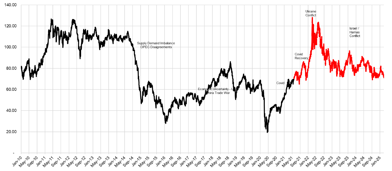
Since 2020, the oil and gas sector has been extremely volatile. For instance, Brent Crude prices surged from a low of USD 20 per barrel in March 2020 to a high of USD 120 per barrel in June 2022, reflecting a sixfold increase in just over 24 months.
Since the June 2022 high, Brent spot prices have declined and reached a new normal of approximately USD 80 per barrel by late 2023. The subsequent price fluctuations have been minimal, as illustrated in the following chart.
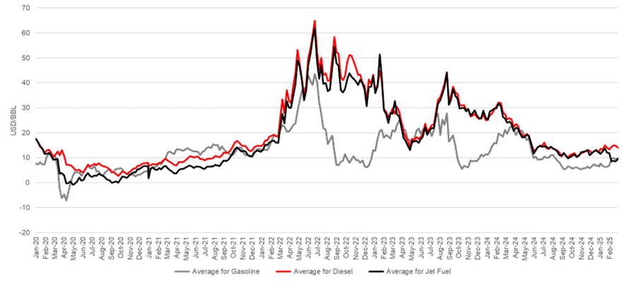
We have also included an extension of crack spreads (the price difference between refined products and crude oil) for the more recent period in the following chart.
The crack spreads followed a similar trend to Brent crude prices, plunging during the pandemic and then surging significantly in 2022. They have generally stabilized since late 2023. Notably, gasoline crack spreads had underperformed compared to diesel and jet fuel. Businesses reliant on diesel and jet fuel must continue operations to meet the demand in transportation, logistics and aviation. In contrast, gasoline demand has lagged due to the shift towards hybrid work environments and the ongoing transition to electric vehicles (EVs).
However, we are now entering a new phase of potential volatility with rising tensions in the Middle East, potential tariffs imposed by the Trump administration, a global economic downturn, and OPEC countries looking to increase market share through higher production. The question remains: will oil prices stabilize around USD 80 per barrel, or will global events reignite volatility?
Sum Insured
From an overarching principal, there are significant benefits to all parties involved in setting the correct sum insured, for instance:
- Insured – Ensures sufficient funds to recover losses
- Insurer – Allows for an accurate premium that reflects the associated risks
- Broker – Secures the correct commission while meeting clients’ expectations in the event of a loss
While this may seem straightforward, achieving the correct sum insured can be challenging, particularly in volatile markets. However, it is precisely during such periods that the insurance market must ensure sums insured are adequately set to avoid surprises for any party involved.
Several mechanisms are in place to help establish the correct sum insured:
- Forward-looking assessments – instead of relying on historical data, commodity price tracking or forward-looking pricing curves can offer a more accurate reflection of future risks, though they may still fall short of real-world conditions.
- Regular asset valuation in response to changes in market conditions.
- Frequent updates to brokers and underwriters to keep all parties aligned with the current risk environment.
At MDD, our experts can collaborate with companies to verify the necessary documentation and assist in preparing accurate sum insured values. Reporting the correct sum insured is essential to help businesses align with the Volatility Clause, ensuring they maintain adequate coverage, even in highly fluctuating market environments.
Volatility Clause
With the Average Clause increasingly being removed from insurance policies, the Volatility Clause was introduced with the aim of protecting insurers against the risks associated with incorrect sum insured values and significant market fluctuations.
On 11 September 2019, LMA5383 was published, making the introduction of the initial Volatility Clause. A little over a year later, on 27 November 2020, LMA5515 was introduced. However, a key complication arose when the Insured experienced a partial interruption, as there was no mechanism to adjust the volatility cap accordingly. As a result, the clause could not provide the intended protection for insurers.
To address this issue, which Insurers found unsuitable for partial losses, LMA5515A was published in March 2024. This updated clause focuses on targeting the policy’s indemnity exposure in the following manner:
- For interruptions equal or less than 10 months from the date of Damage, the Calendar Monthly Cap applicable to each monthly period of the interruption shall apply
- For interruptions greater than 10 months from the date of Damage, the Annual Cap shall apply on a pro-rata basis
- Following Damage, if the (Re)Insured is able to continue / resume with partial operations at the Location(s) suffering Business Interruption loss, then the Caps calculated in 1.1 and 1.2 shall be proportionately reduced by the amount that the Actual Business Results achieved from the partial operations bears as a ratio to the total Expected Business Results at the Location(s) suffering Business Interruption loss. For the avoidance of doubt, the Expected Business Results and Actual Business Results are individually calculated for each Calendar Month or Annual period for which a Cap is to be applied. (Bold by MDD)
The above means that the cap will be adjusted based on a proportionate comparison of the Expected and Actual Business Results, as shown below:

To put this concept into practice, we have applied both LMA5515 and LMA5515A in the following theoretical loss calculations to demonstrate their impact on our loss measurement:
Loss Example 1 Details:
- Date of loss: 1 January 20XX
- Impact: 50% of production impacted
- Indemnity Period: 6 months (max IP 12 months)
- Deductible: 30-day waiting period
- Volatility Clause: 120% of the annual and monthly sum insured.
- Sum Insured: USD 500 million
Since the loss period is less than 10 months, the Volatility Clause directs us to adopts the monthly cap, which equates to USD 50 million (USD 500 million / 12 months x 120%). Under LMA5515, there is no adjustment for partial losses, so we simply compare the USD 50 million cap to the estimated monthly loss to determine whether the monthly cap applies.
Conversely, under LMA5515A, a partial loss adjustment factor is applied (for the purposes of this example, we assume a 50% production shortfall, which directly correlates to a 50% reduction in business results). Therefore, we compare the proportionally adjusted monthly cap (USD 50 million x 50% impact = USD 25 million) to the estimated monthly loss values.
The results of this comparison are summarised in the following table:
| Period | Monthly Loss | LMA5515 | LMA5515A | ||
| Volatility Cap | Net Loss | Volatility Cap | Net Loss | ||
| USD m | USD m | USD m | USD m | USD m | |
| M1 | Waiting Period | Waiting Period | |||
| M2 | 27.0 | 50.0 | 27.0 | 25.0 | 25.0 |
| M3 | 40.0 | 50.0 | 40.0 | 25.0 | 25.0 |
| M4 | 43.0 | 50.0 | 43.0 | 25.0 | 25.0 |
| M5 | 37.0 | 50.0 | 37.0 | 25.0 | 25.0 |
| M6 | 31.0 | 50.0 | 31.0 | 25.0 | 25.0 |
| Total | 178.0 | 178.0 | 125.0 | ||
As illustrated above, the impact is significant, exceeding USD 50 million. It is important to note that the adequacy of the sum insured, if calculated, is approximately 45%.
However, it should be noted that the impact may not be that significant if the sums insured are set correctly and regularly updated to reflect current market conditions. In such cases, the impact may be negligible.
Loss Example 2 Details:
- Date of loss: 1 March 20XX
- Impact: 20% of production impacted
- Indemnity Period: 7 months (max IP 18 months)
- Deductible: 30-day waiting period
- Volatility Clause: 120% of the annual sum insured and 130% of the monthly sum insured
- Sum Insured: USD 360 million
Similar to Loss Example 1, the loss period is less than 10 months, leading us to determine a monthly cap of USD 26 million (USD 360 million / 18 months x 130%). In this example, we assume a 20% production shortfall, translating to a 20% reduction in business results. While LMA5515 does not adjust the cap for partial losses, LMA5515A accounts for them, yielding a proportionally adjusted monthly cap of USD 5.2 million (USD 26 million x 20% impact). We then compare this cap or adjusted cap to the estimated monthly loss values.
The results of this comparison are summarised in the following table:
| Period | Monthly Loss | LMA5515 | LMA5515A | ||
| Volatility Cap | Net Loss | Volatility Cap | Net Loss | ||
| USD m | USD m | USD m | USD m | USD m | |
| M1 | Waiting Period | Waiting Period | |||
| M2 | 4.5 | 26.0 | 4.5 | 5.2 | 4.5 |
| M3 | 5.0 | 26.0 | 5.0 | 5.2 | 5.0 |
| M4 | 3.5 | 26.0 | 3.5 | 5.2 | 3.5 |
| M5 | 3.8 | 26.0 | 3.8 | 5.2 | 3.8 |
| M6 | 4.2 | 26.0 | 4.2 | 5.2 | 4.2 |
| M7 | 4.0 | 26.0 | 4.0 | 5.2 | 4.0 |
| Total | 25.0 | 25.0 | 25.0 | ||
As illustrated above, there is no adjustment to the estimated monthly loss under either clause. If assessed, the adequacy of the sum insured would be approximately 90%. However, with the allowed uplift of 30%, the cap remains well above the estimated monthly loss, ensuring full indemnification of the total loss to the insured.
Conclusion
In recent years, the energy market has witnessed extreme fluctuations, with oil prices swinging dramatically from the lows of 2020 to a significant surge in 2022. While market conditions have somewhat stabilized, ongoing global tensions and economic uncertainties could reignite volatility.
In this unpredictable landscape, LMA5515A introduces timely enhancements to insurance coverage, while allowing for the flexibility necessary in a rapidly changing world.
The key benefits are summarised below:
- A more balanced approach for assessing partial loss scenarios
- Enhanced protection for insurers when the sum insured is adequate
- A level of flexibility for the Insured to manage the unpredictability of market conditions through the use of uplift percentages

Nattakarn Prasitsumrit
ACMA, CGMA, CFE, CVA, Senior Manager
- +65 6327 3785
- nprasitsumrit@mdd.com
- Singapore, APAC


Articles
Relevant Articles
Our experts are extremely knowledgeable about thier subject areas and often write educational material and commentary on topical issues they come across.

Oil, Inflation, and the Dollar: The Global Impact of the Hormuz Crisis
The recent escalation involving Iran has once again drawn global attention to the Strait of Hormuz. This narrow stretch of water plays a critical role in the modern energy system, linking the Persian Gulf to the open ocean via the...

Floatovoltaics – Where Sun Meets Water
Renewable energy has been a source of energy for thousands of years and has been successfully utilized by humans. Most common sources of renewable energy include, but are not limited to, solar, wind, hydro, etc. with hydro energy being most...

Power Generation in the United States – Current Situation
Much has been said in recent times about the ever-increasing need for greater energy supply to meet the growing demand from power-hungry technologies like data centers, artificial intelligence (AI) and electric vehicles (EVs). But how are we faring in the...

Transforming the Petrochemical Landscape
The global energy industry is undergoing a dramatic shift as traditional refining processes evolve to meet the burgeoning demand for petrochemicals while contending with price volatility and environmental mandates. Navigating Global Energy Market Fluctuations The energy sector is no stranger...

Transitioning to Sustainable Power Generation: A Global Perspective
In recent years, the transition to renewable energy has become a central focus for nations across the globe. This movement is driven by the urgent need to address climate change, reduce carbon emissions, and meet the growing energy demands of...

Examining Volatility in the Energy Markets
Introduction In this technical briefing, we aim to provide an update on key Oil and Gas market indices and discuss whether we have moved past the significant volatility experienced between 2020 and 2024, or if the uncertainties persist in the...

Deep-Sea Mining – Panacea or Problem?
For quite some time now, much has been said about the world’s move toward clean energy and the goal toward net zero by 2050. To achieve this, demand will continue to grow for certain critical minerals, such as lithium, nickel,...

How is Electrification Disrupting the Energy Sector?
One of the biggest trends shaping society today is the widespread adoption of Electric Vehicles (EVs). While Tesla pioneered this movement as a disruptor, nearly every automobile manufacturer worldwide is now actively developing its own electric vehicles. Governments have implemented...

Carbon Capture – Is it Really Going to Materialise?
Before we discuss the carbon capture process and how it is used, it is worthwhile conceptualising the carbon emissions emitted worldwide and why different technologies, including carbon capture, must be considered as part of the energy transition. As can be...

Natural Gas – The Past, Present and Future
There has been a significant push towards transitioning to cleaner and renewable energy sources, moving away from fossil fuels due to their environmental impact. By looking at the past, the present and the future, the question remains: can we realistically...

High Grade Ore And A Question Of Indemnity
When a mine suffers business interruption, the issue of high grading can come into play. The question is whether insurers should actually benefit? Mining business interruption insurance and the principle of indemnity is no simple matter. Take the case of...

Recognition of Lost Production at a Gold Mine
With any loss measurement, we must understand how the incident impacted operations. In mining losses, this is no different, we need to understand both mining and milling operations. So, when there is an incident at a mine, how does this...

Renewable Energy Losses – Winds of Change
It is May 20, 1899. New York City taxicab driver Jacob German is the recipient of the United States’ first-ever speeding ticket. He whizzed by at 12 miles per hour on Lexington Avenue and was then pursued and remanded by...
 Losses")
Biomass (Co-Generation) Losses
Certain agricultural entities can generate energy from the organic matter derived from their production process. This type of co-generation of energy is referred to as biomass energy. These biomasses can be agricultural in nature, as in the case of sugarcane...

Variable Mining Costs – How Should They Be Treated?
Variable expenses: one would consider this to be one of the easier aspects in the analysis of a mining claim; however, that is far from the truth. When it comes to mining losses, the determination of which costs are considered...

The Effect of Volatility on Power Generation Business Interruption Losses
It is clear to the casual observer that many aspects of the economy are facing volatility. Fuel, energy, labor, shipping - all have experienced unprecedented shortages and price increases because of a myriad of conditions. The Russia-Ukraine war, Covid-19, inflation,...

Upstream Oil and Gas Losses
In this briefing, we discuss various considerations in upstream oil and gas production losses, and in particular how rates of production depend on the type of well. We also discuss what the shift to horizontal drilling and hydraulic fracturing means...

How is the Power Generation Landscape In Canada Evolving and What Are The Challenges It Faces in the Near Future?
Canada is a world leader in power generation as it pertains to sources that do not emit greenhouse gasses. At the current moment, 83% of generation comes from non-emitting sources. Canada’s goal by 2030 is to have 90% of power...

Back to Coal mining in the UK, what about the risk, which risk?
If you have an interest in energy, heavy industry or simply ESG you cannot fail to have seen the news towards the end of last year - that the UK has approved its first coal mine for many years. The...

Waste to Energy
What is Waste to Energy? Waste to energy refers to the process of converting municipal solid waste (MSW), otherwise known as trash, into usable heat, electricity, or fuel. The three main MSW categories include: Biomass or biogenic (plant or animal...

An Introduction to Natural Gas: Separation, LNG and GTL Plants
Our first technical briefing introduced the Oil & Gas value chain, divided into: i) upstream; ii) midstream; and iii) downstream. Here is a recap, before we explore natural gas in more detail. Upstream: this involves the exploration and extraction of...

Imbalance of Gas Supply
The sanctions imposed on Russia amid the Russia-Ukraine conflict have impacted global gas markets, particularly those in Europe. Russia is the second largest producer of natural gas globally and used to supply about 40% of Europe's natural gas. However, supplies...

Mining BI Insurance: Remediation and Rehabilitation
All mines, no matter how vast or intricate, are ultimately temporary and will one day be depleted. When all valuable materials are extracted, or at least those that are cost-effective, mining operations will cease, and the mine will be decommissioned....
Renewable Energy Certificates
Since 1978, American regulators and policymakers have looked to incentivize the investment and development of generating renewable energy. Individual states began enacting Renewable Portfolio Standards (RPS) to support this mission by requiring a specific percentage of a utility’s energy portfolio...

Mining BI Insurance: Depreciation, Depletion and Amortization
The use of depreciation, depletion and amortization (DD&A) is an accounting method that allows the cost of an asset to be recorded as an expense over a period of time in order to reflect the use and consumption of the...

Potential Quantification Issues for Losses Involving Wind Farms Under Construction
Quantifying the financial impact stemming from the failure of an already commissioned single stand-alone wind turbine generator presents challenges, but these challenges increase exponentially when the failure occurs at a wind farm under construction. Additional complexities surface to the extent...

The Global Energy Crisis
As the Ukrainian conflict unfolds, Europe’s energy dependence on Russia becomes an increasingly critical bargaining tool. The economic sanctions imposed by some Western nations in response to Russia’s invasion appear to be increasingly directed against Russian oil and gas supplies...

Measuring Refining Margins for a BI Loss
When it comes to Business Interruption policies for Oil & Gas risks, there are different types of coverage available in the market, including Gross Profit, Gross Earnings, Specified Standing Charges etc. Common Policy Wordings Gross Profit equates to Turnover less...

The Importance of Mining Plans
Any well-run business starts with a plan, and a mining operation is no exception. Plans and budgeting or forecasting allow management to prepare for a future period, whether in the short-term or in the long run. Based on projections, management...
 in Refinery Claims")
The Importance of Linear Programs (LPs) in Refinery Claims
The use of Linear Program models is common in refining, and other industries, to optimise their activities by using an algorithm subject to a set of inputs, constraints, and relationships. This article discusses the LP models in more detail and...

What Happened to Jet Fuel During Covid-19?
The main types of jet fuels used by airlines are Jet A-1, Jet A and Jet B. Jet A is mainly used in the United States, whereas Jet A-1 is commonly used outside the United States and Jet B is...

Mining BI Insurance and the Impact of Changes in Ore Grade
Ore grade refers to the metal content of an ore deposit, and it is the value of the contained metals or minerals less the cost of extracting and refining that drives the economics of a mine site. There can be...

A Lightning Fast Intro to Energy Market Basics
The summer has come to an end in Florida. Temperatures are still hot, and the afternoon thunderstorms are raging. So, when I open my electricity bill and gasp at the month’s cost, muttering some hopeless comments about how I should...

The Recovery of Oil & Gas: A Roller Coaster Ride or Merely a Few Speed Bumps?
Covid-19 has led to major disruptions across various sectors and the petroleum industry is no exception. Demand for oil and petroleum products, in general, declined due to reduced economic activity as governments worldwide imposed lockdowns and tightened border controls. Certain...

What Triggered the UK Energy Market Crisis and What is the Impact on BI Claims?
The UK’s energy wholesale markets have reached new highs, with daily average electricity prices rising above GBP 150 per MWh since early September 2021. A record high of GBP 424 per MWh, since at least January 2019, was reached on...
Introduction to the Oil & Gas Value Chain
The Oil and Gas industry in the insurance market is usually categorised between Onshore/Offshore or Upstream/Downstream. It includes a chain of businesses relating to extraction, transportation, refining, petrochemical and chemical – essentially from the carbon in the ground to the...

Regulated and Deregulated Electricity Markets: What is the difference when modelling power generation losses?
Introduction When modelling power generation losses for Business Interruption (“BI”) or Delay in Start-Up (“DSU”) purposes, it is important to understand the type of market(s) the Insured participates in and specifically how it operates within those markets. In this introductory...
Mining Claim – All Is Not As It Appears
In this briefing we focus on mining claims, and share our knowledge and technical expertise on one of the loss measurement issues regularly encountered in mining claims, production bottlenecks. What you will learn from reading the article include: How the...

Mining Business Interruption Insurance and the Principle of Indemnity
Mining Business Interruption Insurance and the Principle of Indemnity A contradiction? How can a mine claim for lost production when the ore is not lost and will be mined? Why does a mining company need to purchase business interruption insurance...

The Effect of Deductibles & Policy Wording – Is It What You Think?
With a typical Energy claim standing at approximately USD 4.5 million, it’s no surprise that Business Interruption (BI) is once again the #1 business risk for the fourth year in a row[i]. To help insurers mitigate their exposure when an...

Court Breaks with Apportionment
The case of Varco Canada Limited v. Pason Systems Corp., 2013 FC 750 (CanLII) involved an award of over $52M based on an accounting of the defendant’s profits. Perhaps more importantly, the decision sheds light on a number of conceptual...

Mining Industry Revisits Anti-Corruption Procedures
Mining companies should take note of Canada’s stricter penalties and more aggressive enforcement of anti-corruption laws and make sure their anti-bribery compliance procedures are up to speed, lawyers, forensic accountants and mining executives warned at a recent conference in Toronto....
